distribute
distribute is a relatively simple command line utility for distributing compute jobs across the powerful
lab computers. In essence, distribute provides a simple way to automatically schedule dozens of jobs
from different people across the small number of powerful computers in the lab.
Besides having the configuration files begin easier to use, distribute also contains a mechanism for
only scheduling your jobs on nodes that meet your criteria. If you require OpenFoam to run your simulation,
distribute automatically knows which of the three computers it can run the job on. This also allows you
to robustly choose what your requirements are for your tasks. This allows us to prioritize
use of the gpu machine to jobs requiring a gpu, increasing the overall throughput of jobs between all lab
members.
Another cool feature of distribute is that files that are not needed after each compute run are automatically
wiped from the hard drive, preserving limited disk space on the compute machines. Files that are specified to be
saved (by you) are archived automatically on a 24 TB storage machine, and can be retrieved (and filtered)
to your personal computer with a single short command.
distribute competes in the same space as slurm, which you would
likely find on an actual compute cluster. The benefit of distribute is an all-in-one solution to running,
archiving, and scheduling jobs with a single streamlined utility without messing around with the complexities
of the (very detailed) slurm documentation. If you are still unconvinced, take a look at the overall architecture
diagram that slurm provides:
Since the lab computers also function as day-to-day workstations for some lab members, some additional
features are required to ensure that they are functional outside of running jobs. distribute solves this issue
by allowing a user that is sitting at a computer to temporarily pause the currently executing job so that
they may perform some simple work. This allows lab members to still quickly iterate on ideas without waiting
hours for their jobs to reach the front of the queue. Since cluster computers are never used as
day-to-day workstations, popular compute schedulers like slurm don't provision for this.
Architecture
Instead of complex scheduling algorithms and job queues, we can distill the overall architecture of the system to a simple diagram:

In summary, there is a very simple flow of information from the server to the nodes, and from the nodes to the server. The server is charged with sending the nodes any user-specified files (such as initial conditions, solver input files, or csv's of information) as well as instructions on how to compile and run the project. Once the job has finished, the user's script will move any and all files that they wish to archive to a special directory. All files in the special directory will be transfered to the server and saved indefinitely.
The archiving structure of distribute helps free up disk space on your laptop of workstation, and instead
keep large files (that will surely be useful at a later date) stored away on a purpose-build machine to
hold them. As long as your are connected to the university network - VPN or otherwise - you can access the
files dumped by your compute job at any time.
Specifying Jobs
We have thus far talked about all the cool things we can do with distribute, but none of this is free. As
a famous Italian engineer once said, "Theres no such thing as free lunch." The largest complexity with working
with distribute is the configuration file that specifies how to compile run project. distribute template python
will generate the following file:
meta:
  batch_name: your_jobset_name
  namespace: example_namespace
  matrix: ~
  capabilities:
    - gfortran
    - python3
    - apptainer
python:
  initialize:
    build_file: /path/to/build.py
  jobs:
    - name: job_1
      file: execute_job.py
    - name: job_2
      file: execute_job_2.py
We will explain all of these fields later, but surmise it to say that the configuration files come in 3 main sections.
The meta section will describe things that the head node must do, including what "capabilities" each node is required
to have to run your server, a batch_name and namespace so that your compute results do not overwrite someone else's,
and a matrix field so that you can specify an optional matrix username that will be pinged once all your
jobs have finished.
The next section is the initialize section. This section specifies all the files and instructions that are required
to compile your project before it is run. This step is kept separate from the running step so that we can ensure
that your project is compiled only once before being run with different jobs in the third section.
The third section tells distribute how to execute each job. If you are using a python configuration then your
file parameter will likely seek out the compiled binary from the second step and run the binary using whatever
files you chose to be available.
The specifics of the configuration file will be discussed in greater detail in a later section.
Installation
In order to install distribute you must have a recent version of rustc and cargo.
Install instructions can be found here.
Once you have it (and running cargo shows some output), you can install the project with
cargo install --git https://github.com/fluid-Dynamics-Group/distribute --force
and you are good to go! If you run into any trouble installing, let Brooks know.
Python api install
pip3 install distribute_compute_config
Command Basics
There are a few commands that you will need to know to effectively work with distribute. Don't worry,
they are not too complex. The full list of commands and their specific parameters can be found by running
$ distribute
at the time of writing, this yields:
distribute 0.9.4
A utility for scheduling jobs on a cluster

USAGE:
    distribute [FLAGS] <SUBCOMMAND>

FLAGS:
    -h, --help         Prints help information
        --save-log
        --show-logs
    -V, --version      Prints version information

SUBCOMMANDS:
    add              add a job set to the queue
    client           start this workstation as a node and prepare it for a server connection
    help             Prints this message or the help of the given subcommand(s)
    kill             terminate any running jobs of a given batch name and remove the batch from the queue
    node-status      check the status of all the nodes
    pause            pause all currently running processes on this node for a specified amount of time
    pull             Pull files from the server to your machine
    run              run a apptainer configuration file locally (without sending it off to a server)
    server           start serving jobs out to nodes using the provied configuration file
    server-status    check the status of all the nodes
    template         generate a template file to fill for executing with `distribute add`
add
distribute add is how you can add jobs to the server queue. There are two main things needed to operate this command:
a configuration file and the IP of the main server node. If you do not specify the name of a configuration
file, it will default to distribute-jobs.yaml. This command can be run (for most cases) as such:
distribute add --ip <server ip address here> my-distribute-jobs-file.yaml
or, using defaults:
distribute add --ip <server ip address here>
If there exists no node that matches all of your required capabilities, the job will not be run. There also exists a --dry flag
if you want to check that your configuration file syntax is correct, and a --show-caps flag to print the capabilities
of each node.
template
distribute template is a simple way to create a distribute-jobs.yaml file that either runs with python or apptainers. The specifics
of each configuration file will be discussed later.
distribute template python
---
meta:
  batch_name: your_jobset_name
  namespace: example_namespace
  matrix: ~
  capabilities:
    - gfortran
    - python3
    - apptainer
python:
  initialize:
    build_file: /path/to/build.py
    required_files:
      - path: /file/always/present/1.txt
        alias: optional_alias.txt
      - path: /another/file/2.json
        alias: ~
      - path: /maybe/python/utils_file.py
        alias: ~
  jobs:
    - name: job_1
      file: execute_job.py
      required_files:
        - path: job_configuration_file.json
          alias: ~
        - path: job_configuration_file_with_alias.json
          alias: input.json
and
distribute template apptainer
---
meta:
  batch_name: your_jobset_name
  namespace: example_namespace
  matrix: ~
  capabilities:
    - gfortran
    - python3
    - apptainer
apptainer:
  initialize:
    sif: execute_container.sif
    required_files:
      - path: /file/always/present/1.txt
        alias: optional_alias.txt
      - path: /another/file/2.json
        alias: ~
      - path: /maybe/python/utils_file.py
        alias: ~
    required_mounts:
      - /path/inside/container/to/mount
  jobs:
    - name: job_1
      required_files:
        - path: job_configuration_file.json
          alias: ~
        - path: job_configuration_file_with_alias.json
          alias: input.json
pause
If you use a compute node as a work station, distribute pause will pause all locally running jobs so that you
can use the workstation normally. It takes a simple argument as an upper bound on how long the tasks can be paused. The maximum amount of time that
a job can be paused is four hours (4h), but if this is not enough you can simply rerun the command. This
upper bound is just present to remove any chance of you accidentally leaving the jobs paused for an extended
period of time.
If you decide that you no longer need the tasks paused, you can simply Ctrl-C to quit the hanging command
and all processes will be automatically resumed. Do not close your terminal before the pausing finishes or
you have canceled it with Ctrl-C as the job on your machine will never resume.
some examples of this command:
sudo distribute pause --duration 4h
sudo distribute pause --duration 1h30m10s
sudo distribute pause --duration 60s
server-status
distribute status prints out all the running jobs at the head node. It will show you all the job batches
that are currently running, as well as the number of jobs in that set currently running and the
names of the jobs that have not been run yet. You can use this command to fetch the required parameters
to execute the kill command if needed.
distribute server-status --ip <server ip here>
If there is no output then there are no jobs currently in the queue or executing on nodes.
TODO An example output here
260sec
        :jobs running now: 1
10sec_positive
        -unforced_viscous_decay
        -unforced_inviscid_decay
        -viscous_forcing_no_compensation_eh_first
        -viscous_forcing_no_compensation_eh_second
        -viscous_forcing_no_compensation_eh_both
        :jobs running now: 0
pull
distribute pull takes a distribute-jobs.yaml config file and pulls all the files associated with that batch
to a specified --save-dir (default is the current directory). This is really convenient because the only thing
you need to fetch your files is the original file you used to compute the results in the first place!
Since you often dont want to pull all the files - which might include tens or hundreds of gigabytes of flowfield
files - this command also accepts include or exclude filters, which consist of a list of regular expressions
to apply to the file path. If using a include query, any file matching one of the regexs will be pulled to
your machine. If using a exclude query, any file matching a regex will not be pulled to your computer.
The full documentation on regular expressions is found here, but luckily
most character strings are valid regular exprssions (barring characters like +, -, (, )). Lets say your
meta section of the config file looks like this:
---
meta:
  batch_name: incompressible_5second_cases
  namespace: brooks_openfoam_cases
  capabilities: []
and your directory tree looks something like this
├── incompressible_5second_cases
    ├── case1
    │   ├── flowfield.vtk
    │   └── statistics.csv
    ├── case2
    │   ├── flowfield.vtk
    │   └── statistics.csv
    └── case3
        ├── flowfield.vtk
        └── statistics.csv
If you wanted to exclude any file with a vtk extension, you could
distribute pull distribute-jobs.yaml --ip <server ip here> \
	exclude \
		--exclude "vtk"
Or, if you wanted to exclude all of the case3 files and all vtk files:
distribute pull distribute-jobs.yaml --ip <server ip here> \
	exclude \
		--exclude "vtk" \
		--exclude "case3"
Maybe you only want to pull case1 files:
distribute pull distribute-jobs.yaml --ip <server ip here> \
	include \
		--include "case1"
run
distribute run will run an apptainer job locally. It is usefull for debugging apptainer jobs
since the exact commands that are passed to the container are not always intuitive.
distribute run --help
distribute-run 0.6.0
run a apptainer configuration file locally (without sending it off to a server)

USAGE:
    distribute run [FLAGS] [OPTIONS] [job-file]

FLAGS:
        --clean-save    allow the save_dir to exist, but remove all the contents of it before executing the code
    -h, --help          Prints help information
    -V, --version       Prints version information

OPTIONS:
    -s, --save-dir <save-dir>    the directory where all the work will be performed [default: ./distribute-run]

ARGS:
    <job-file>    location of your configuration file [default: distribute-jobs.yaml]
An example is provided in the apptainer jobs section.
Configuration
Configuration files are fundamental to how distribute works. Without a configuration file, the server would not
know what nodes that jobs could be run on, or even what the content of each job is. Configuration files
are also useful in pulling the files you want from your compute job to your local machine. Therefore,
they are imperative to understand.
Configuration files
As mentioned in the introduction, configuration files (usually named distribute-jobs.yaml) come in two flavors:
python scripts and apptainer images.
The advantage of python scripts is that they are relatively easy to produce: you need to have a single script that specifies how to build your project, and another script (for each job) that specifies how to run each file. The disadvantage of python configurations is that they are very brittle - the exact server configuration may be slightly different from your environment and therefore can fail in unpredictable ways. Since all nodes with your capabilities are treated equally, a node failing to execute your files will quickly chew through your jobs and spit out some errors.
The advantage of apptainer jobs is that you can be sure that the way the job is run
on distribute nodes is exactly how it would run on your local machine. This means that, while it may take
slightly longer to make a apptainer job, you can directly ensure that all the dependencies are present, and that there wont
be any unexpected differences in the environment to ruin your job execution. The importance of this cannot be
understated. The other advantage of apptainer jobs is that they can be directly run on other compute clusters (as
well as every lab machine), and they are much easier to debug if you want to hand off the project to another lab
member for help. The disadvantage of apptainer jobs is that the file system is not mutable - you cannot write
to any files in the the container. Any attempt to write a file in the apptainer filesystem will result in an error
and the job will fail. Fear not, the fix for this is relatively easy: you will just bind folders from the host file system
(via configuration file) to your container that will be writeable. All you have to do then is ensure that your
compute job only writes to folders that have been bound to the container from the host filesystem.
Regardless of using a python or apptainer configuration, the three main areas of the configuration file remain the same:
| Section | Python Configuration | Apptainer Configuration |
|---|---|---|
| Meta |
|
The same as python |
| Building |
|
|
| Running |
|
|
How files are saved
Files are saved on the server using your namespace, batch_name, and job_names. Take the following configuration file that specifies
a apptainer job that does not save any of its own files:
meta:
  batch_name: example_jobset_name
  namespace: example_namespace
  matrix: @your-username:matrix.org
  capabilities: []
apptainer:
  initialize:
    sif: execute_container.sif
    required_files: []
    required_mounts:
      - /path/inside/container/to/mount
  jobs:
    - name: job_1
      required_files: []
    - name: job_2
      required_files: []
    - name: job_3
      required_files: []
The resulting folder structure on the head node will be
.
└── example_namespace
    └── example_jobset_name
        ├── example_jobset_name_build_ouput-node-1.txt
        ├── example_jobset_name_build_ouput-node-2.txt
        ├── example_jobset_name_build_ouput-node-3.txt
        ├── job_1
        │   └── stdout.txt
        ├── job_2
        │   └── stdout.txt
        └── job_3
            └── stdout.txt
The nice thing about distribute is that you also receive the output that would appear on your terminal
as a text file. Namely, you will have text files for how your project was compiled (example_jobset_name_build_ouput-node-1.txt
is the python build script output for node-1), as well as the output for each job inside each respective folder.
If you were to execute another configuration file using a different batch name, like this:
meta:
  batch_name: example_jobset_name
  namespace: example_namespace
  matrix: @your-username:matrix.org
  capabilities: []

# -- snip -- #
the output would look like this:
.
└── example_namespace
    ├── another_jobset
    │   ├── example_jobset_name_build_ouput-node-1.txt
    │   ├── example_jobset_name_build_ouput-node-2.txt
    │   ├── example_jobset_name_build_ouput-node-3.txt
    │   ├── job_1
    │   │   └── stdout.txt
    │   ├── job_2
    │   │   └── stdout.txt
    │   └── job_3
    │       └── stdout.txt
    └── example_jobset_name
        ├── example_jobset_name_build_ouput-node-1.txt
        ├── example_jobset_name_build_ouput-node-2.txt
        ├── example_jobset_name_build_ouput-node-3.txt
        ├── job_1
        │   └── stdout.txt
        ├── job_2
        │   └── stdout.txt
        └── job_3
            └── stdout.txt
Therefore, its important to ensure that your batch_name fields are unique. If you don't, the output of
the previous batch will be deleted or combined with the new job.
Examples
Examples creating each configuration file can be found in the current page's subchapters.
Python
Python configuration file templates can be generated as follows:
distribute template python
At the time of writing, it outputs something like this:
---
meta:
  batch_name: your_jobset_name
  namespace: example_namespace
  matrix: ~
  capabilities:
    - gfortran
    - python3
    - apptainer
python:
  initialize:
    build_file: /path/to/build.py
    required_files:
      - path: /file/always/present/1.txt
        alias: optional_alias.txt
      - path: /another/file/2.json
        alias: ~
      - path: /maybe/python/utils_file.py
        alias: ~
  jobs:
    - name: job_1
      file: execute_job.py
      required_files:
        - path: job_configuration_file.json
          alias: ~
        - path: job_configuration_file_with_alias.json
          alias: input.json
What You Are Provided
You may ask, what do your see when they are executed on a node? While the base folder structure remains the same, the files you are provided differ. Lets say you are executing the following section of a configuration file:
python:
  initialize:
    build_file: /path/to/build.py
    required_files:
      - path: file1.txt
      - path: file999.txt
        alias: file2.txt
  jobs:
    - name: job_1
      file: execute_job.py
      required_files:
        - path: file3.txt
    - name: job_2
      file: execute_job.py
      required_files: []
When executing the compilation, the folder structure would look like this:
.
├── build.py
├── distribute_save
├── initial_files
│   ├── file1.txt
│   └── file2.txt
└── input
    ├── file1.txt
    ├── file2.txt
In other words: when building you only have access to the files from the required_files section in initialize. Another thing
to note is that even though you have specified the path to the file999.txt file on your local computer, the file has actually
been named file2.txt on the node. This is an additional feature to help your job execution scripts work uniform file names; you
dont actually need to need to keep a bunch of solver inputs named solver_input.json in separate folders to prevent name collision.
You can instead have several inputs solver_input_1.json, solver_input_2.json, solver_input_3.json on your local machine and
then set the alias filed to solver_input.json so that you run script can simply read the file at ./input/solver_input.json!
Lets say your python build script (which has been renamed to build.py by distribute for uniformity) clones the STREAmS solver
repository and compiled the project. Then, when executing job_1 your folder structure would look something like this:
.
├── job.py
├── distribute_save
├── initial_files
│   ├── file1.txt
│   └── file2.txt
├── input
│   ├── file1.txt
│   ├── file2.txt
│   └── file3.txt
└── STREAmS
    ├── README.md
    └── src
        └── main.f90
Now, the folder structure is exactly as you have left it, plus the addition of a new file3.txt that you specified in your required_files
section under jobs. Since job_2 does not specify any additional required_files, the directory structure when running the python
script would look like this:
.
├── job.py
├── distribute_save
├── initial_files
│   ├── file1.txt
│   └── file2.txt
├── input
│   ├── file1.txt
│   ├── file2.txt
└── STREAmS
    ├── README.md
    └── src
        └── main.f90
In general, the presence of ./initial_files is an implementation detail. The files in this section are not refreshed
between job executions. You should not rely on the existance of this folder - or modify any of the contents of it. The
contents of the folder are copied to ./input with every new job; use those files instead.
Saving results of your compute jobs
Archiving jobs to the head node is super easy. All you have to do is ensure that your execution script moves all files
you wish to save to the ./distribute_save folder before exiting. distribute will automatically read all the files
in ./distribute_save and save them to the corresponding job folder on the head node permenantly. distribute will
also clear out the ./distribute_save folder for you between jobs so that you dont end up with duplicate files.
Build Scripts
The build script is specified in the initialize section under the build_file key. The build script is simply responsible
for cloning relevant git repositories and compiling any scripts in the project. Since private repositories require
a github SSH key, a read-only ssh key is provided on the system so that you can clone any private fluid-dynamics-group
repo. An example build script that I have personally used for working with hit3d looks like this:
import subprocess
import os
import sys
import shutil
# hit3d_helpers is a python script that I have specified in
# my `required_files` section of `initialize`
from initial_files import hit3d_helpers
import traceback

HIT3D = "https://github.com/Fluid-Dynamics-Group/hit3d.git"
HIT3D_UTILS = "https://github.com/Fluid-Dynamics-Group/hit3d-utils.git"
VTK = "https://github.com/Fluid-Dynamics-Group/vtk.git"
VTK_ANALYSIS = "https://github.com/Fluid-Dynamics-Group/vtk-analysis.git"
FOURIER = "https://github.com/Fluid-Dynamics-Group/fourier-analysis.git"
GRADIENT = "https://github.com/Fluid-Dynamics-Group/ndarray-gradient.git"
DIST = "https://github.com/Fluid-Dynamics-Group/distribute.git"
NOTIFY = "https://github.com/Fluid-Dynamics-Group/matrix-notify.git"

# executes a command as if you were typing it in a terminal
def run_shell_command(command):
    print(f"running {command}")
    output = subprocess.run(command,shell=True, check=True)
    if not output.stdout is None:
        print(output.stdout)

# construct a `git clone` string to run as a shell command
def make_clone_url(ssh_url, branch=None):
    if branch is not None:
        return f"git clone -b {branch} {ssh_url} --depth 1"
    else:
        return f"git clone {ssh_url} --depth 1"

def main():
    build = hit3d_helpers.Build.load_json("./initial_files")

    print("input files:")
    run_shell_command(make_clone_url(HIT3D, build.hit3d_branch))
    run_shell_command(make_clone_url(HIT3D_UTILS, build.hit3d_utils_branch))
    run_shell_command(make_clone_url(VTK))
    run_shell_command(make_clone_url(VTK_ANALYSIS))
    run_shell_command(make_clone_url(FOURIER))
    run_shell_command(make_clone_url(GRADIENT))
    run_shell_command(make_clone_url(DIST, "cancel-tasks"))
    run_shell_command(make_clone_url(NOTIFY))

    # move the directory for book keeping purposes
    shutil.move("fourier-analysis", "fourier")

    # build hit3d
    os.chdir("hit3d/src")
    run_shell_command("make")
    os.chdir("../../")

    # build hit3d-utils
    os.chdir("hit3d-utils")
    run_shell_command("cargo install --path .")
    os.chdir("../")

    # build vtk-analysis
    os.chdir("vtk-analysis")
    run_shell_command("cargo install --path .")
    os.chdir("../")

    # all the other projects cloned are dependencies of the built projects
    # they don't need to be explicitly built themselves

if __name__ == "__main__":
    main()
note that os.chdir is the equivalent of the GNU coreutils cd command: it simply changes the current working
directory.
Job Execution Scripts
Execution scripts are specified in the file key of a list item a job name in jobs. Execution scripts
can do a lot of things. I have found it productive to write a single generic_run.py script that
reads a configuration file from ./input/input.json is spefied under my required_files for the job)
and then run the sovler from there.
One import thing about execution scripts is that they are run with a command line argument specifying how many cores you are allowed to use. If you hardcode the number of cores you use you will either oversaturate the processor (therefore slowing down the overall execution speed), or undersaturate the resources available on the machine. Your script will be "executed" as if it was a command line program. If the computer had 16 cores available, this would be the command:
python3 ./job.py 16
you can parse this value using the sys.argv value in your script:
import sys
allowed_processors = sys.argv[1]
allowed_processors_int = int(allowed_processors)
assert(allowed_processors_int, 16)
You must ensure that you use all available cores on the machine. If your code can only use a reduced number
of cores, make sure you specify this in your capabilities section! Do not run single threaded
processes on the distributed computing network - they will not go faster.
A full working example of a run script that I use is this:
import os
import sys
import json
from input import hit3d_helpers
import shutil
import traceback

IC_SPEC_NAME = "initial_condition_espec.pkg"
IC_WRK_NAME = "initial_condition_wrk.pkg"

def load_json():
    path = "./input/input.json"

    with open(path, 'r') as f:
        data = json.load(f)
        print(data)
        return data

# copies some initial condition files from ./input
# to the ./hit3d/src directory so they can be used
# by the solver
def move_wrk_files(is_root):
	outfile = "hit3d/src/"
	infile = "input/"

    shutil.copy(infile + IC_SPEC_NAME, outfile + IC_SPEC_NAME)
    shutil.copy(infile + IC_WRK_NAME, outfile + IC_WRK_NAME)


# copy the ./input/input.json file to the output directory
# so that we can see it later when we download the data for viewing
def copy_input_json(is_root):
	outfile = "distribute_save/"
	infile = "input/"

    shutil.copy(infile  + "input.json", outfile + "input.json")

if __name__ == "__main__":
    try:
        data = load_json();

        # get the number of cores that we are allowed to use from the command line
        nprocs = int(sys.argv[1])

        print(f"running with nprocs = ", nprocs)

        # parse the json data into parameters to run the solver with
        skip_diffusion = data["skip_diffusion"]
        size = data["size"]
        dt = data["dt"]
        steps = data["steps"]
        restarts = data["restarts"]
        reynolds_number = data["reynolds_number"]
        path = data["path"]
        load_initial_data = data["load_initial_data"]
        export_vtk = data["export_vtk"]
        epsilon1 = data["epsilon1"]
        epsilon2 = data["epsilon2"]
        restart_time = data["restart_time"]
        skip_steps = data["skip_steps"]
        scalar_type = data["scalar_type"]
        validate_viscous_compensation = data["validate_viscous_compensation"]
        viscous_compensation = data["viscous_compensation"]
        require_forcing = data["require_forcing"]
        io_steps = data["io_steps"]
        export_divergence = data["export_divergence"]

		# if we need initial condition data then we copy it into ./hit3d/src/
        if not load_initial_data == 1:
            move_wrk_files()

        root = os.getcwd()

        # open hit3d folder
        openhit3d(is_root)

		# run the solver using the `hit3d_helpers` file that we have
		# ensured is present from `required_files`
        hit3d_helpers.RunCase(
            skip_diffusion,
            size,
            dt,
            steps,
            restarts,
            reynolds_number,
            path,
            load_initial_data,
            nprocs,
            export_vtk,
            epsilon1,
            epsilon2,
            restart_time,
            skip_steps,
            scalar_type,
            validate_viscous_compensation,
            viscous_compensation,
            require_forcing,
            io_steps,
            export_divergence
        ).run(0)

        # go back to main folder that we started in
        os.chdir(root)

        copy_input_json(is_root)

        sys.exit(0)

    # this section will ensure that the exception and traceback
	# is printed to the console (and therefore appears in stdout files saved
	# on the server
    except Exception as e:
        print("EXCEPTION occured:\n",e)
        print(e.__cause__)
        print(e.__context__)
        traceback.print_exc()
        sys.exit(1)
Full Example
A simpler example of a python job has been compiled and verified here.
Apptainer
Apptainer (previously named Singularity) is a container system often used for packaging HPC applications. For us,
apptainer is useful for distributing your compute jobs since you can specify the exact dependencies required
for running. If your container runs on your machine, it will run on the distributed cluster!
As mentioned in the introduction, you must ensure that your container does not write to any directories that are not bound by the host system. This will be discussed further below, but suffice it to say that writing to apptainer's immutable filesystem will crash your compute job.
Versus Docker
There is an official documentation page discussing the differences between docker
and apptainer here. There a few primary
benefits for using apptainer from an implementation standpoint in distribute:
- Its easy to use GPU compute from apptainer
- Apptainer compiles down to a single
.siffile that can easily be sent to thedistributeserver and passed to compute nodes - Once your code has been packaged in apptainer, it is very easy to run it on paid HPC clusters
Overview of Apptainer configuration files
Apptainer definition files
This documentation is not the place to discuss the intricacies of apptainer. As a user, we have tried to make
it as easy as possible to build an image that can run on distribute.
The apptainer-common was purpose built to give you a good
starting place with compilers and runtimes (including fortran, C++, openfoam, python3). Your definition file
needs to look something like this:
Bootstrap: library
From: library://vanillabrooks/default/fluid-dynamics-common

%files from build
    # in here you copy files / directories from your host machine into the
	# container so that they may be accessed and compiled.
	# the sintax is:

	/path/to/host/file /path/to/container/file

%post
    # install any extra packages required here
	# possibly with apt, or maybe pip3

%apprun distribute
    # execute your solver here
	# this section is called from a compute node
A (simplified) example of a definition file I have used is this:
Bootstrap: library
From: library://vanillabrooks/default/fluid-dynamics-common

%files
	# copy over my files
	/home/brooks/github/hit3d/ /hit3d
	/home/brooks/github/hit3d-utils/ /hit3d-utils
	/home/brooks/github/vtk/ /vtk
	/home/brooks/github/vtk-analysis/ /vtk-analysis
	/home/brooks/github/fourier/ /fourier
	/home/brooks/github/ndarray-gradient/ /ndarray-gradient
	/home/brooks/github/matrix-notify/ /matrix-notify
	/home/brooks/github/distribute/ /distribute

%environment
	CARGO_TARGET_DIR="/target"

%post
	# add cargo to the environment
	export PATH="$PATH":"$HOME/.cargo/bin"

	cd /hit3d-utils
	cargo install --path .
	ls -al /hit3d-utils

	cd /hit3d/src
	make

	cd /vtk-analysis
	cargo install --path .

	# move the binaries we just installed to the root
	mv $HOME/.cargo/bin/hit3d-utils /hit3d/src
	mv $HOME/.cargo/bin/vtk-analysis /hit3d/src

	#
	# remove directories that just take up space
	#
	rm -rf /hit3d/.git
	rm -rf /hit3d/target/
	rm -rf /hit3d/src/output/
	rm -rf /hit3d-utils/.git
	rm -rf /hit3d-utils/target/

	#
	# simplify some directories
	#
	mv /hit3d/src/hit3d.x /hit3d.x

	# copy the binaries to the root
	mv /hit3d/src/vtk-analysis /vtk-analysis-exe
	mv /hit3d/src/hit3d-utils /hit3d-utils-exe

	mv /hit3d-utils/plots /plots

	mv /hit3d-utils/generic_run.py /run.py

%apprun distribute
	cd /
	python3 /run.py $1
I want to emphasize one specific thing from this file: the %apprun distribute section is very important. On a node
with 16 cores, your distribute section gets called like this:
apptainer run --app distribute 16
In reality, this call is actually slightly more complex (see below), but this command is illustrative of the point. You must ensure you pass the number of allowed cores down to whatever run script you are using. In our example:
%apprun distribute
	cd /
	python3 /run.py $1
We make sure to pass down the 16 we received with $1 which corresponds to "the first argument that this bash script was
called with". Similar to the python configuration, your python file is also responsible for parsing this value and running
your solver with the appropriate number of cores. You can parse the $1 value you pass to python using the sys.argv value
in your script:
import sys
allowed_processors = sys.argv[1]
allowed_processors_int = int(allowed_processors)
assert(allowed_processors_int, 16)
You must ensure that you use all available cores on the machine. If your code can only use a reduced number
of cores, make sure you specify this in your capabilities section! Do not run single threaded
processes on the distributed computing network - they will not go faster.
Full documentation on apptainer definition files can be found on the official site. If you are building an apptainer image based on nvidia HPC resources, your header would look something like this (nvidia documentation):
Bootstrap: docker
From: nvcr.io/nvidia/nvhpc:22.1-devel-cuda_multi-ubuntu20.05
Building Apptainer Images
Compiling an apptainer definition file to a .sif file to run on the distribute compute is relatively simple (on linux). Run something like this:
mkdir ~/apptainer
APPTAINER_TMPDIR="~/apptainer" sudo -E apptainer build your-output-file.sif build.apptainer
where your-output-file.sif is the desired name of the .sif file that apptainer will spit out, and build.apptainer is the
definition file you have built. The APPTAINER_TMPDIR="~/apptainer" portion of the command sets the APPTAINER_TMPDIR environment
variable to a location on disk (~/apptainer) because apptainer / apptainer can often require more memory to compile the sif file
than what is available on your computer (yes, more than your 64 GB). Since apptainer build requires root privileges, it must be run with sudo. The additional
-E passed to sudo copies the environment variables from the host shell (which is needed for APPTAINER_TMPDIR)
Binding Volumes (Mutable Filesystems)
In order for your compute job to do meaningful work, you will likely save some files. But we know that apptainer image files are not mutable. The answer to this problem is binding volumes. A "volume" is container-language for a folder inside the container that actually corresponds to a folder on the host system. Since these special folders ("volumes") are actually part of the host computer's filesystem they can be written to without error. The process of mapping a folder in your container to a folder on the host system is called "binding".
With apptainer, the binding of volumes to a container happens at runtime. Since distribute wants you to have
access to a folder to save things to (in python: ./distribute_save), as well as a folder to read the required_files
you specified (in python: ./distribute_save). Apptainer makes these folders slightly easier to access by binding them
to the root directory: /distribute_save and /input. When running your apptainer on the compute node with 16
cores, the following command is used to ensure that these bindings happen:
apptainer run apptainer_file.sif --app distribute --bind \
	path/to/a/folder:/distribute_save:rw,\
	path/to/another/folder:/input:rw\
	16
Note that the binding arguments are simply a comma separated list in the format folder_on_host:folder_in_container:rw
where rw specifies that files in the folder are readable and writeable.
If your configuration file for apptainer looks like this:
meta:
  batch_name: your_jobset_name
  namespace: example_namespace
  capabilities: []
apptainer:
  initialize:
    sif: execute_container.sif
    required_files:
      - path: file1.txt
      - path: file999.txt
        alias: file2.txt
    required_mounts: []
  jobs:
    - name: job_1
      required_files:
        - path: file3.txt
    - name: job_2
      required_files: []
When running job_1, the /input folder looks like this:
input
├── file1.txt
├── file2.txt
└── file3.txt
And when running job_2, the /input folder looks like this:
input
├── file1.txt
├── file2.txt
For a more detailed explanation of this behavior read the python configuration documentation.
Now a natural question you may have is this: If volume bindings are specified at runtime - and not
within my apptainer definition file - how can I possibly get additional mutable folders? Am I stuck
with writing to /input and /distribute_save? The answer is no! You can tell distribute what folders
in your container you want to be mutable with the required_mounts key in the initialize section of
your configuration. For example, in the hit3d solver (whose definition file is used as the example
above), the following folder structure at / would be present at runtime:
.
├── distribute_save
├── hit3d-utils-exe
├── hit3d.x
├── input
├── plots
│   ├── energy_helicity.py
│   ├── proposal_plots.py
│   └── viscous_dissapation.py
└── vtk-analysis-exe
However, hit3d requires a folder called output relative to itself. Since this folder is required,
we might be (naively) tempted to simply add a call to mkdir /output in our %post section of the
definition file. However, we would then be creating an immutable directory within the image. Instead,
we simply just need to add this path to our configuration file:
meta:
  batch_name: your_jobset_name
  namespace: example_namespace
  capabilities: []
apptainer:
  initialize:
    sif: execute_container.sif
    required_files:
      - path: file1.txt
      - path: file999.txt
        alias: file2.txt
    required_mounts:
	  - /output				# <---- here
  jobs:
    - name: job_1
      required_files:
        - path: file3.txt
    - name: job_2
      required_files: []
By adding this line, your container will be invoked like this (on a 16 core machine):
apptainer run apptainer_file.sif --app distribute --bind \
	path/to/a/folder:/distribute_save:rw,\
	path/to/another/folder:/input:rw,\
	path/to/yet/another/folder/:/output:rw\
	16
Configuration File
A default configuration file can be generated with :
distribute template apptainer
---
meta:
  batch_name: your_jobset_name
  namespace: example_namespace
  matrix: ~
  capabilities:
    - gfortran
    - python3
    - apptainer
apptainer:
  initialize:
    sif: execute_container.sif
    required_files:
      - path: /file/always/present/1.txt
        alias: optional_alias.txt
      - path: /another/file/2.json
        alias: ~
      - path: /maybe/python/utils_file.py
        alias: ~
    required_mounts:
      - /path/inside/container/to/mount
  jobs:
    - name: job_1
      required_files:
        - path: job_configuration_file.json
          alias: ~
        - path: job_configuration_file_with_alias.json
          alias: input.json
The meta section is identical to the meta section of python. For apptainer configurations, the only
capability you need to specify is apptainer or apptainer. If you require your job to use a gpu,
you can also specify a gpu capability.
The initialize section takes in a single .sif file
that is built using the apptainer build command on a definition file, as well as some files that you always want
to be available in the /input directory. Then, the required_mounts provides a way to bind mutable directories
to the inside of the container. Make sure that the directory you are binding to does not actually exist in the container
(but its parent directory does exist).
The job section is also very similar to the python configuration, but instead of taking python scripts and some files
that should be present on the system, it exclusively takes required_files that should be present. This is discussed
more in the next section.
Workflow Differences From Python
The largest difference you will encounter between the apptainer and python configurations is the way in
which they are executed. While each python job has its own file that it may use for execution, the apptainer
workflow simply relies on whatever occurs in %apprun distribute to read files from /input and execute the
binary directly. Therefore, each job in the configuration file only operates on some additional input files
and the .sif file never changes. This is slightly less flexible than the python configuration (which allows
for individual python files to run each job), but by storing your input files in some intermediate structure
(like json) this difficulty can be easily overcome.
Debugging Apptainer Jobs / Example
Because there are a lot of ways that your job might go wrong, you can use the distribute run command
to run an apptainer configuration file in place. As an example, take this test
that is required to compile and run in the project. The apptainer definition file is:
Bootstrap: library
From: ubuntu:20.04

%files
	./run.py /run.py

%post
	apt-get update -y
	apt install python3 -y

%apprun distribute
    cd /
    python3 /run.py $1
run.py is:
import sys

def main():
    procs = int(sys.argv[1])
    print(f"running with {procs} processors")

    print("writing to /dir1")
    with open("/dir1/file1.txt", "w") as f:
        f.write("checking mutability of file system")

    print("writing to /dir2")
    with open("/dir2/file2.txt", "w") as f:
        f.write("checking mutability of file system")

    # read some input files from /input

    print("reading input files")
    with open("/input/input.txt", "r") as f:
        text = f.read()
        num = int(text)

    with open("/distribute_save/simulated_output.txt", "w") as f:
        square = num * num
        f.write(f"the square of the input was {square}")

if __name__ == "__main__":
    main()
input_1.txt is:
10
input_2.txt is:
15
and distribute-jobs.yaml is:
---
meta:
  batch_name: some_batch
  namespace: some_namespace
  capabilities: []
apptainer:
  initialize:
    sif: apptainer_local.sif
    required_files: []
    required_mounts:
      - /dir1
      - /dir2
  jobs:
    - name: job_1
      required_files:
        - path: input_1.txt
          alias: input.txt
    - name: job_2
      required_files:
        - path: input_2.txt
          alias: input.txt
the apptainer definition file can be built with these instructions. Then, execute the job locally:
distribute run distribute-jobs.yaml --save-dir output --clean-save
The output directory structure looks like this:
output
├── archived_files
│   ├── job_1
│   │   ├── job_1_output.txt
│   │   └── simulated_output.txt
│   └── job_2
│       ├── job_2_output.txt
│       └── simulated_output.txt
├── _bind_path_0
│   └── file1.txt
├── _bind_path_1
│   └── file2.txt
├── distribute_save
├── initial_files
├── input
│   └── input.txt
└── apptainer_file.sif
This shows that we were able to write to additional folders on the host system (_bind_path_x), as well as read and write output files. Its worth noting that
if this job was run on the distributed server, it would not be archived the same (archive_files directory is simply a way to save distribute_save without
deleting data). The structure on the server would look like this:
some_namespace
├── some_batch
    ├── job_1
    │   ├── job_1_output.txt
    │   └── simulated_output.txt
    └── job_2
        ├── job_2_output.txt
        └── simulated_output.txt
The outputs of the two simulated_output.txt files are:
the square of the input was 100
and
the square of the input was 225
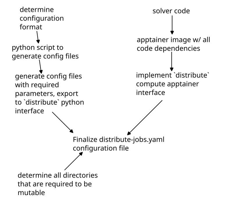
Python Api
Since solver configuration files are sometimes machine generated, it can be arduous to manually create
distribute-jobs.yaml files with methods like distribute template. To aid in this difficulty, a python
package is available to generate configurations with minimal effort.
Full Documentation
Detailed documentation is found here
Available Capabilities
Current capabilities of nodes in our lab are tracked as an example file in the repository. There are a few things to take away from this file:
Capabilities for Apptainer jobs
The only required capability for an apptainer job is apptainer.
All dependencies and requirements can be handled by you in the apptainer definition file.
Excluding Certain Machines from Executing Your Job
While any machine can run your jobs if they match the capabilities, sometimes you wish to avoid a machine
if you know that someone will be running cases locally (not through the distributed system) and will simply
distribute pause your jobs - delaying the finish for your batch.
To account for this possibility, you can add a capability lab1 to only run the job on the lab1 machine, lab2 to only
run on lab2, etc. If you simply dont want to run on lab3, then you can specify lab1-2. Likewise, you can skip lab1 with
lab2-3.
Machines
| name | physical core count | address | role |
|---|---|---|---|
| lab1 | 16 | 134.197.94.134 | compute |
| lab2 | 16 | 134.197.27.105 | compute |
| lab3 | 32 | 134.197.95.113 | compute |
| lab4 | 12 | 134.197.94.155 | storage |
| lab5 | 32 | 134.197.27.69 | compute |
| distserver | 12 | 134.197.95.21 | head node |
- If you are adding a job with
distribute add, you should usedistserverip address. - If you are updating the
distributesource code on all machines, you should uselab1,lab2,lab3anddistserverlab4server must be accessed through a FreeBSD jail